10 Data Wrangling and Cleaning (Part II)
In this session, we are going to learn how to clean more challenging data than what we encountered in the last chapter. In contrast to the last chapter, this section is more of a reference guide than an end-to-end cleaning example. That’s because the tools you learn here might not always pop up, or at least are unlikely to all pop up in the one data frame. Nonetheless, when you combine the functions you learn here to clean data with the functions from last week, you will be able to handle an impressive amount (probably around 80%) of any data cleaning challenges you will encounter in your research.
By the end of this session, you should be capable of the following:
Understand the concepts of wide and long data and be capable of
pivoting(i.e., transforming) from one format to another.Know how to merge together separate data frames into one file that you can clean.
Identifying and handling missing data (
NAvalues).
10.1 Let’s Get Set Up
Similar to the last chapter, first we need to set up RStudio and download some data files.
10.1.1 Activity 1.1: Set up your WD
Remember that the working directory is the location where we want to store any resulting data files or scripts that you’ll work on in a session. In Chapter 2, I showed you how to do this using a button-and-click interface.
Using those instructions, create a folder called “Week11” in the rintro project folder (or whatever folder you created) and set it as your working directory. Use the getwd() to check that it has been set as your working directory. Your output should be something like this:
10.1.2 Activity 1.2: Import your CSV files and R script
You need to import several files for this activity:
background.csv
flanker_task1.csv
flanker_task2.csv
flanker_task3.csv
demographics.csv
reaction_time.csv
raw_remote_clean.csv
You can find this files either on Canvas or on the OSF Page.
If you’re using RStudio, you should see these files in your working directory within the Files pane. Create an R script and save it as (data_cleaning_ii_script.R).
To import the raw_remote_associations.csv dataset into R, do the following:
- Click Environment in the Environment Pane -> Import Dataset -> From Text(base) -> Select demographics.csv -> change its name to df_dem
- Click Environment in the Environment Pane -> Import Dataset -> From Text(base) -> Select flanker_task1.csv -> change its name to df_flanker1
- Click Environment in the Environment Pane -> Import Dataset -> From Text(base) -> Select flanker_task2.csv -> change its name to df_flanker2
- Click Environment in the Environment Pane -> Import Dataset -> From Text(base) -> Select flanker_task3.csv -> change its name to df_flanker3
- Follow the same instructions to import the demographics.csv, reaction_time.csv, and raw_remote_clean.csv files. Change their name to df_demographics, df_rt, and df_clean respectively.
- See Chapter 4’s section on importing data for more information
Alternatively, you can write and run the following commands within the data_cleaning_ii_script.R. Just make sure they are in the Week 11 folder and that you have set that folder as your working directory.
10.2 Data Formats (Long and Wide Data)
Psychological research often involves working with data stored in tables, commonly referred to as Data Frames. These tables can take two primary formats: wide or long. Depending on the research software used, the raw data downloaded from a study might be in either wide or long table format.
Understanding the differences between these formats is crucial because each format facilitates certain tasks more easily. Similarly, knowing how to effectively and efficiently pivot (i.e., transform or convert) between these formats is essential for performing specific tasks on the data. Fortunately, R and the tidyverse package are well-equipped to handle both types of data and to convert between them seamlessly.
In this section, we will first define wide and long data formats and discuss the advantages of each format over its counterpart. We will then explore how to pivot between these formats using R.
10.2.1 Defining Long and Wide Data
Wide Data
In wide data, each row represents a unique participant, and each column represents a separate variable. Table 6.1 shows an example of data in wide format. Each row contains all the information on a specific participant across each variable collected. For example, in one row of information, we can observe that participant 2 is 25 years old, 165 centimeters tall, weighs 60kg, and has a BMI score of 22.
| ID | Age | Height | Weight | BMI |
|---|---|---|---|---|
| 1 | 30 | 175 | 76 | 24.8 |
| 2 | 25 | 165 | 60 | 22 |
| 3 | 35 | 185 | 80 | 23.4 |
If you are like most psychologists, you are used to seeing data in wide formats. Data is often inputted in wide format in software like Excel or SPSS, as it easier for humans to read. We are used to scanning data horizontally (left-right) rather than vertically (up-down). Because each participant is in a single row, repetition in the data frame is minimized, again making it easier for us to read..
In terms of statistical analysis, wide data is useful for calculating descriptive statistics (e.g., mean, standard deviations) on variables. Certain statistical tests like ANOVA, Linear Regression, and Correlation are easier to compute in R when the data is in wide format.
Long Data
In long data, each row contains a participant’s single response to a single variable. The table below illustrates data in long format. Instead of having a column for each variable, there is one column that identifies the measured variable, and another column contains the participant’s response to that variable. If multiple variables are collected, each participant has several rows, with each row representing a single response to a single variable.
| ID | Variable | Value |
|---|---|---|
| 1 | Age | 30 |
| 1 | Height | 175 |
| 1 | Weight | 76 |
| 1 | BMI | 24.8 |
| 2 | Age | 25 |
| 2 | Height | 165 |
| 2 | Weight | 60 |
| 2 | BMI | 22 |
| 3 | Age | 35 |
| 3 | Height | 185 |
| 3 | Weight | 80 |
| 3 | BMI | 23.4 |
Each row in Table 6.2 represents a participant’s response to a single variable. For example, in row 1, we see that participant 1 reported their age (Variable) as 30 (Value). But I have to look to other rows to see this participant’s score on other variables.
It is more difficult to scan long data to quickly capture the information that we need. However, it is often easier for computers and programming languages to work with long data. This is one of the reasons why the concept of Tidy Data discussed in the previous chapter prefers data in the long format - every row contains the minimum amount of information needed rather than “cluttering” rows with lots of information.
This preference for long data isn’t only stylistic, long-data format is more suitable for certain forms of analyses. Long data is often more suitable if you are analyzing data in R that involves repeated measures or longitudinal designs, basically any test where we are interested in within-subject variability over time. Similarly, a lot of the packages/functions developed to enable high quality data visualizations were built with the assumption that your data is in long-format.
10.3 Converting the Format of Our Data
While it’s important to know the differences between wide and long data formats, do not feel you have to memories every detail. If you are running a statistical test it’ll be pretty easy to find out what type of format your data needs to be in. If the data is not in the correct format, then the tidyverse package makes it straightforward to convert one format to another, thanks to two functions called: pivot_longer() and pivot_wider().
10.3.1 Pivoting from Wide to Long
The pivot_longer() function converts a wide data frame into long format. Typing ?pivot_longer into the console provides detailed information about this function in RStudio through the Help tab in the Files Pane7.
There is a lot of information that will appear in the help section. I want to draw your attention to the Usage section, which contains the arguments (inputs) that we can specify in the pivot_longer() function.
There is a lot of potential inputs we can throw in, but I want to highlight the key arguments that you will use most of the time when you use this function
| Argument | Meaning |
|---|---|
data |
Here you specify the wide data frame that you want to convert to long format |
cols |
The column(s) that will be moved or altered when you pivot the data frame. |
names_to |
The names of each variable identified in cols will be stored in a new column in our long data frame. The names_to argument specifies the name(s) of that new column(s). |
values_to |
The values associated with each variable identified in cols will be stored in a new column in our long data frame. The values_to argument specifies the name of that new column. |
Let’s create an example data frame to use pivot_longer()longer with. I recommend you copy and paste the code below to your R script and run it to create the data frame
#set.seed(123) ensures that the data my R generates will be the same as the data your R generates. This is because the function rnorm() used below randomly generates numbers.

set.seed(123)


wide_df <- data.frame(
  ID = 1:10,
  Wellbeing = round(rnorm(n = 10, mean = 4, sd = 0.8), 2),
  Extraversion = round(rnorm(n = 10, mean = 3, sd = 0.8), 2),
  Neuroticism = round(rnorm(n = 10, mean = 3, sd = 0.8), 2),
  Conscientiousness = round(rnorm(n = 10, mean = 3, sd = 0.8), 2),
  Openness = round(rnorm(n = 10, mean = 3, sd = 0.8), 2)
)

#rnorm() randomly generates a set of numbers (n) that have a certain mean and standard deviation. I put this function inside round() to set the number of decimal places.

head(wide_df)
## ID Wellbeing Extraversion Neuroticism Conscientiousness Openness
## 1 1 3.55 3.98 2.15 3.34 2.44
## 2 2 3.82 3.29 2.83 2.76 2.83
## 3 3 5.25 3.32 2.18 3.72 1.99
## 4 4 4.06 3.09 2.42 3.70 4.74
## 5 5 4.10 2.56 2.50 3.66 3.97
## 6 6 5.37 4.43 1.65 3.55 2.10So we’ve created a wide data frame with 10 participants (5 male, 5 female) with scores on each of the Big Five personality traits. We know the data frame is wide because every variable is a separate column and each row tells us a participant’s response to each variable.
Let’s see how we can convert this data frame from wide to long using pivot_longer(). We’ll call the long data frame long_df:
long_df <- pivot_longer(
  wide_df,
  cols = Wellbeing:Openness, #we will pivot everything except ID
  names_to = "Variable",
  values_to = "Response"
)

head(long_df)
## # A tibble: 6 × 3
## ID Variable Response
## <int> <chr> <dbl>
## 1 1 Wellbeing 3.55
## 2 1 Extraversion 3.98
## 3 1 Neuroticism 2.15
## 4 1 Conscientiousness 3.34
## 5 1 Openness 2.44
## 6 2 Wellbeing 3.82Now we have the same data frame but in a different format.
The figure below gives an example of the pivot process. We typically do not pivot the ID column, because that enables us to identify which participant’s score each variable. Let’s look at what happens if we do include ID in the cols argument
## # A tibble: 60 × 2
##    name              Response
##    <chr>                <dbl>
##  1 ID                    1
##  2 Wellbeing             3.55
##  3 Extraversion          3.98
##  4 Neuroticism           2.15
##  5 Conscientiousness     3.34
##  6 Openness              2.44
##  7 ID                    2
##  8 Wellbeing             3.82
##  9 Extraversion          3.29
## 10 Neuroticism           2.83
## # ℹ 50 more rows
Now we have lost our record for identifying which participant contributed to which data point. This identifies a key about using pivot_longer() in that not EVERYTHING needs to pivoted, it depends on our analytical needs are. Let’s go through a slightly more complicated data frame to illustrate what I mean by this.
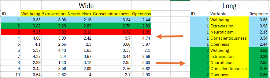
Figure 10.1: Visual representation of what is pivoted
10.3.2 Pivoting our Remote Associations Data Frame
Last week, we cleaned the raw_remote_associations.csv data frame and stored it in a variable called df_clean. If we use head(), we’ll see that it’s in wide format.
#if you do not have df_clean in your environment, download the dataset `raw_remote_clean.csv` from the Teams channel, and put in the week 5 folder.

#Run the following code to load it in
#df_clean <- read.csv("raw_remote_clean.csv")

head(df_clean)
## ID condition age gender remote_pos remote_neg remote_neut total_mood
## 1 10229436 CAB 26 male 0 2 4 61
## 2 10230533 CAB 36 female 0 4 4 62
## 3 10230659 ABC 45 female 0 5 0 74
## 4 10428518 BCA 37 male 0 9 9 68
## 5 10229522 CAB 30 female 1 1 0 59
## 6 10229414 ABC 36 female 1 1 1 63
## total_openness mean_openness
## 1 16 3.2
## 2 15 3.0
## 3 17 3.4
## 4 14 2.8
## 5 16 3.2
## 6 14 2.8Let’s convert df_clean to the long data format, and let’s call it df_clean_long. However, we are not going to follow the same protocol as the last example, where we pivoted everything except ID. For this data frame, we are going to include every variable inside the cols argument except for ID, condition, and gender.
df_clean_long <- pivot_longer(df_clean,
  cols = c(age, remote_pos:mean_openness), #we select age, and then we select everything from remote_pos to mean_openness in df_clean
  names_to = "Variable", #this creates a column called `variables` that will tell us the the variable the participant provided data for
  values_to = "Response"#this creates a column called `answer` that will tell us participants actual answer to each variable
)


print(df_clean_long)
## # A tibble: 266 × 5
## ID condition gender Variable Response
## <int> <chr> <chr> <chr> <dbl>
## 1 10229436 CAB male age 26
## 2 10229436 CAB male remote_pos 0
## 3 10229436 CAB male remote_neg 2
## 4 10229436 CAB male remote_neut 4
## 5 10229436 CAB male total_mood 61
## 6 10229436 CAB male total_openness 16
## 7 10229436 CAB male mean_openness 3.2
## 8 10230533 CAB female age 36
## 9 10230533 CAB female remote_pos 0
## 10 10230533 CAB female remote_neg 4
## # ℹ 256 more rowsThere we have it! Now our data is in long format. Each row contains a participant’s individual score on a particular variable. But this time, the participant’s information on condition and gender also gets replicated for each row created for that participant.
But why did we not include the variables condition and gender in our conversion? There are both technical and analytical reasons for this decision. Let’s address the technical reason first.
Technically, we actually can’t create the Answer column by combining participants responses on variables like condition and gender with their answers on the other variables. This is because the data type for both condition and gender are factors, whereas the data type for every other variable is numeric.
If you remember from our vector discussion (and remember everything that every column is just a lucky vector who found a home) we mentioned that vectors are lines of data where everything in the line is of the same data type. You can have character vectors, factor vectors, numerical vectors, logical vectors, integer vectors, but you cannot have a single vector with multiple data types.
So if we try pivot_longer on our df_clean data frame, including the gender and condition columns, we get the following error:
pivot_longer(df_clean,
  cols = c(condition:mean_openness), #we try to select everything except ID
  names_to = "Variable", #this creates a column called `variables` that will tell us the the variable the participant provided data for
  values_to = "Response"#this creates a column called `answer` that will tell us participants actual answer to each variable
)
## Error in `pivot_longer()`:
## ! Can't combine `condition` <character> and `age` <integer>.If you’re stubborn and you insist on pivoting everything, then you would need to convert all of our columns to the same data type. There is an argument in the pivot_longer() function that enables us to do this, called values_transform. The easiest solution would be to transform everything that will go into our Response vector/column into a character.
pivot_longer(df_clean,
  cols = condition:mean_openness,
  names_to = "Variable",
  values_to = "Response",
  values_transform = list(Response = as.character) #takes everything that will be put into the Response column and uses the `as.character()` function on it.
  )
## # A tibble: 342 × 3
## ID Variable Response
## <int> <chr> <chr>
## 1 10229436 condition CAB
## 2 10229436 age 26
## 3 10229436 gender male
## 4 10229436 remote_pos 0
## 5 10229436 remote_neg 2
## 6 10229436 remote_neut 4
## 7 10229436 total_mood 61
## 8 10229436 total_openness 16
## 9 10229436 mean_openness 3.2
## 10 10230533 condition CAB
## # ℹ 332 more rowsThat creates an example of a long data frame, which looks neater than our earlier attempt. However, I don’t recommend this approach. Since everything inside Response is not a character, we can’t conduct any quantitative analysis, defeating the purpose.
This leads me on to the analytical reason why we don’t want to pivot our condition and gender columns. Since condition and gender are factors, we’’ want to investigate the extent to which participants scores on Wellbeing and our Big Five traits are influenced by that factor. In other words, we want to investigate the effect of our independent variables on our dependent variables. If you look at df_clean_long, the data frame keeps a record of a participant’s score on each dependent variable in relation to our two independent variables. This sets us up nicely for conducting statistical analysis.
## # A tibble: 10 × 5
##          ID condition gender Variable       Response
##       <int> <chr>     <chr>  <chr>             <dbl>
##  1 10229436 CAB       male   age                26
##  2 10229436 CAB       male   remote_pos          0
##  3 10229436 CAB       male   remote_neg          2
##  4 10229436 CAB       male   remote_neut         4
##  5 10229436 CAB       male   total_mood         61
##  6 10229436 CAB       male   total_openness     16
##  7 10229436 CAB       male   mean_openness       3.2
##  8 10230533 CAB       female age                36
##  9 10230533 CAB       female remote_pos          0
## 10 10230533 CAB       female remote_neg          4
10.3.3 Pivoting from Long to Wide
Now that we’ve covered converting data frames from wide to long, how can we convert from long to wide? We can use the pivot_wider() function. The figure below shows the results of typing ?pivot_wider into the console. The table below it shows the key arguments of this function.
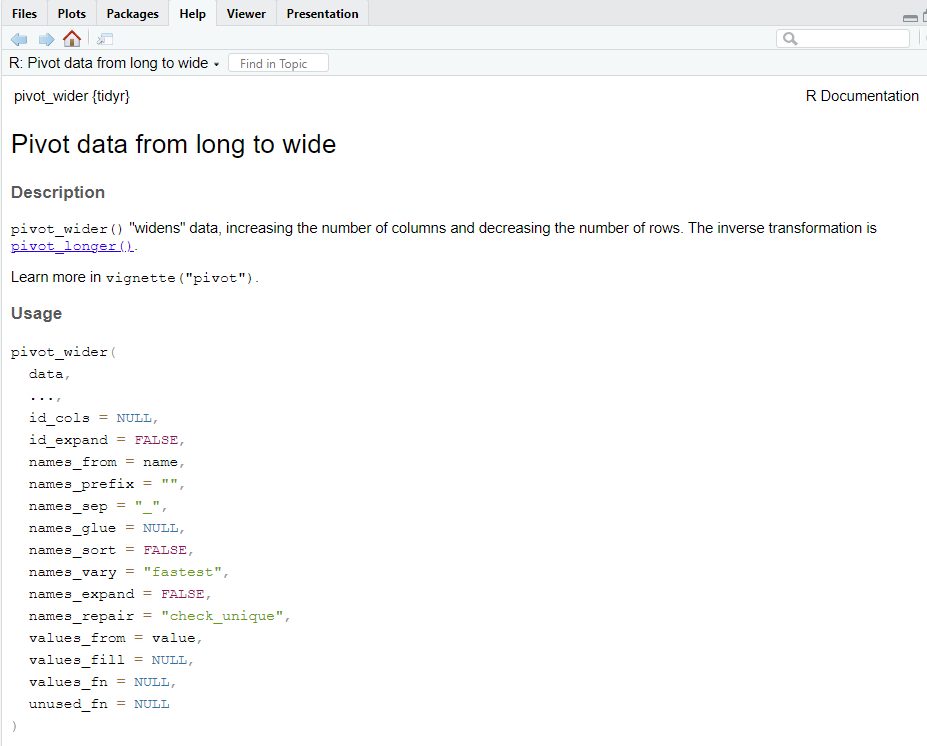
Figure 10.2: The arguments that we can pass to the pivot_wider() function
| Argument | Meaning |
|---|---|
data |
The long data frame that you want to convert to wide format |
id_cols |
The columns that help identify each participant. This is often the values that are repeated in each row within a long data frame (e.g., like ID or any independent variables) |
names_from |
When we pivot from long to wide, we will be creating new columns for each variable that we collected data on. We need to tell R where to find the names for those variables. |
values_from |
We need to tell R where to find the values for the new columns that we are creating. |
Let’s use pivot_wider() to convert our long_df back into wide format.
## # A tibble: 10 × 6
##       ID Wellbeing Extraversion Neuroticism Conscientiousness Openness
##    <int>     <dbl>        <dbl>       <dbl>             <dbl>    <dbl>
##  1     1      3.55         3.98        2.15              3.34     2.44
##  2     2      3.82         3.29        2.83              2.76     2.83
##  3     3      5.25         3.32        2.18              3.72     1.99
##  4     4      4.06         3.09        2.42              3.7      4.74
##  5     5      4.1          2.56        2.5               3.66     3.97
##  6     6      5.37         4.43        1.65              3.55     2.1
##  7     7      4.37         3.4         3.67              3.44     2.68
##  8     8      2.99         1.43        3.12              2.95     2.63
##  9     9      3.45         3.56        2.09              2.76     3.62
## 10    10      3.64         2.62        4                 2.7      2.93
Look familiar? If you compare it to our original wide_df, you’ll notice they look exactly the same.
Now let’s do the same thing with the long version of remote_associations data frame.
df_clean_wide <- pivot_wider(df_clean_long,
                             id_cols = ID:gender,
                             names_from = Variable,
                             values_from = Response)

head(df_clean_wide)
## # A tibble: 6 × 10
## ID condition gender age remote_pos remote_neg remote_neut total_mood
## <int> <chr> <chr> <dbl> <dbl> <dbl> <dbl> <dbl>
## 1 10229436 CAB male 26 0 2 4 61
## 2 10230533 CAB female 36 0 4 4 62
## 3 10230659 ABC female 45 0 5 0 74
## 4 10428518 BCA male 37 0 9 9 68
## 5 10229522 CAB female 30 1 1 0 59
## 6 10229414 ABC female 36 1 1 1 63
## # ℹ 2 more variables: total_openness <dbl>, mean_openness <dbl>If you compare that to the head of df_clean, you’ll see that its back to the format we cleaned it to last week.
10.3.3.1 Summary
That covers basic pivoting from long to wide and wide to long using pivot_long() and pivot_wide(). However, both functions enable you to handle much more complicated data frames and clean them up as you go. We won’t cover that in this version of the textbook, but I highly recommend reading the Advanced Pivoting section from the Data Wrangling Standford ebook if your pivoting needs are more complicated than the examples here.
10.4 Handling Missing Values
In psychological research, dealing with missing data is a common challenge that requires careful consideration to ensure the integrity and validity of analyses. In this section, we’ll explore how to handle missing values (NA) in R using the tidyverse package. We’ll cover techniques for identifying missing values, strategies for handling them, and best practices for addressing missing data in psychological research studies.
10.4.1 Introduction to Missing Values
Missing values, often represented as NA in R, occur when data is not available or cannot be recorded for certain observations. This can occur due to various reasons such as non-response in surveys, data entry errors, or incomplete data collection processes. It’s essential to understand and address missing values appropriately to avoid biased or misleading results in data analysis.
10.4.2 Identifying Missing Values
Detecting missing values in datasets is the first step towards handling them effectively. In R, we can use functions like is.na() to identify missing values.
# Example dataset with missing values
missing_data <- data.frame(
  id = 1:10,
  age = c(25, NA, 30, 28, 35, NA, 40, 22, NA, 29),
  gender = c("Male", "Female", "Male", NA, "Female", "Male", NA, "Male", "Female", NA)
)

#check for missing values
missing_values <- summarise_all(missing_data, ~sum(is.na(.)))

#inside summarise_all, we tell R to pick the missing_data and then to sum up the number of missing values inside that data frame.

print(missing_values)
## id age gender
## 1 0 3 3In this example, we’ve created a dataset missing_data with variables age and gender, some of which contain missing values. We then used summarise_all() along with is.na() to count the number of missing values in each column.
We can see that there are three missing values in both the age and gendernder columns.
10.4.3 Removing Missing Values
To remove rows or columns with missing values, we can use functions like drop_na() or na.omit() in the tidyverse. Here’s how we can remove rows with missing values in the age column:
# Remove rows with missing values in the age column
removed_data <- drop_na(missing_data)

print(removed_data)
## id age gender
## 1 1 25 Male
## 2 3 30 Male
## 3 5 35 Female
## 4 8 22 Male## id age gender
## 1 1 25 Male
## 3 3 30 Male
## 5 5 35 Female
## 8 8 22 Male10.5 Merging Data (i.e., Joining Different Datasets Together)
In psychological research, we’ll often encounter situations where data from multiple sources or studies need to be combined for analysis. We might have collected demographic information separately from participants answers on experimental tasks. We may have collected data using a variety of platforms (e.g., survey data using Qualtrics and response data using PsychoPy). Additionally, the research software tools we use might modulate the data. For example, if we run a study in Gorilla Research, then each separate task and questionnaire gets downloaded as separate files.
Whatever the reason, you will often need to merge or join data together from different sources in order to conduct the analysis you need. Luckily, R is quite capable at facilitating data merging. In this subsection, we will look at ways you can merge different data frames together.
10.5.1 Introduction to Merging Data
Merging data involves combining data frames based on their common variables. Let’s image we have two data frames called df_demographics and df_rt. These data frames contain information on both participants demographic information and their reaction time on a specific task and which condition they were randomly assigned to. Let’s load both of these data frames into R (make sure you have downloaded them and put them into your working directory before running the following code).
Ideally, we would have one merged data frame that would contain a participant’s response on all our variables. However, there are some complications with these two data frames. If you check the number of rows in each data frame, we can see there are differing number of participants.
## [1] 60## [1] 42There are 60 participants in the demographics data frame whereas there are only 42 participants in the reaction time data frame. If the study was online, maybe participants gave up after completing the demographic information, maybe there was connection issues, maybe the data did not save correctly. Whatever the reason for this mismatch in participants, we need to account for this when we merge these data frames together.
Luckily, there are a multitude in ways we can do this through the tidyverse package.
These types of join are:
Inner Join: Includes only the rows that have matching values in both datasets. This type of join retains only the observations that exist in both datasets, excluding unmatched rows.
Left Join: Includes all rows from the left dataset and matching rows from the right dataset. Unmatched rows from the right dataset are filled with NA values.
Right Join: Includes all rows from the right dataset and matching rows from the left dataset. Unmatched rows from the left dataset are filled with NA values.
Outer Join (or Full Join): Includes all rows from both datasets, filling in missing values with NA where there are no matches.
Using our df_demographics and df_rt data frames, lets show you the result of each of these joins and why/when you would use them.
10.5.2 Inner_Join
The inner_join() function joins together two data frames, but it will only keep the rows that have matching values in both data frames.
When we use inner_join() we need to specify the value(s) that we want to match across both data frames. Once we do, then in the case of the df_demographics and df_rt data frames, what this means is that only the participants who match on that specified value(s) in both data frames will merged together.
Let’s create a merged data frame using inner_join and call it df_inner. The syntax for inner_join is: inner_join(df1, df2, by = join_by(column(s))
##           ID     gender age   condition mean_rt
## 1 EoYncPX1QK     Female  24 no caffeine     269
## 2 Zn1yzAeYA4 Non-Binary  21 no caffeine     206
## 3 B4iCIhzgPi       Male  24 no caffeine     187
## 4 9sJnqQM0lo     Female  23 no caffeine     217
## 5 FPSgiOjwA7 Non-Binary  23 no caffeine     160
## 6 0g0AFLyHCe       Male  24 no caffeine     255
We can see that our df_inner has combined the gender and age columns from df_demographics with the condition and mean_rt columns from df_rt. When we use inner_join the order in which specify the data frames is the order in which the columns will be added. So if we wanted the condition and mean_rt columns to come first, then we can change the order:
##            ID     condition mean_rt     gender age
## 1  EoYncPX1QK   no caffeine     269     Female  24
## 2  Zn1yzAeYA4   no caffeine     206 Non-Binary  21
## 3  B4iCIhzgPi   no caffeine     187       Male  24
## 4  9sJnqQM0lo   no caffeine     217     Female  23
## 5  FPSgiOjwA7   no caffeine     160 Non-Binary  23
## 6  0g0AFLyHCe   no caffeine     255       Male  24
## 7  hlmrG4AyLu   no caffeine     145     Female  22
## 8  oOUz7EpZDf   no caffeine     240 Non-Binary  24
## 9  QhvvMEVq1X   no caffeine     212       Male  24
## 10 WHdme1YyZv   no caffeine     207     Female  22
## 11 yFTywINVDl   no caffeine     236 Non-Binary  24
## 12 E4TDInCFgc   no caffeine     157       Male  23
## 13 w15ouKhYjX   no caffeine     139     Female  24
## 14 PRHjvltTq9   no caffeine     185 Non-Binary  23
## 15 T1INTYDoxW  low caffeine     261       Male  23
## 16 wQgCowzLTF  low caffeine     229     Female  22
## 17 gAPefpxFu2  low caffeine     314 Non-Binary  23
## 18 kJRT78syM1  low caffeine     150       Male  24
## 19 zigHVms3ZU  low caffeine     205     Female  23
## 20 MdaNDDZypx  low caffeine     353 Non-Binary  24
## 21 1kVtNcCJZR  low caffeine     201       Male  21
## 22 vWP6tk42hT  low caffeine     245     Female  23
## 23 uSbQmTf4hR  low caffeine     242 Non-Binary  24
## 24 F5JS8n0pw8  low caffeine     281       Male  24
## 25 GNNjyhr80i  low caffeine     203     Female  22
## 26 gg587jx1wz  low caffeine     260 Non-Binary  22
## 27 QG48CYj01m  low caffeine     113       Male  22
## 28 QkyZzgywzF  low caffeine     162     Female  23
## 29 t8x4iOKwnT high caffeine     204 Non-Binary  22
## 30 fAazPW5qCz high caffeine     170       Male  23
## 31 Aug70zOtfX high caffeine     211     Female  22
## 32 DECqK4tIyT high caffeine     114 Non-Binary  23
## 33 GbdjGe0yh2 high caffeine     227       Male  24
## 34 yuSrPEfg8O high caffeine     175     Female  24
## 35 Vq0SB0N0gt high caffeine     177 Non-Binary  23
## 36 rCqGbWbmxW high caffeine     192       Male  22
## 37 crbKl4mP8f high caffeine     171     Female  22
## 38 PPL7VpIJAA high caffeine     114 Non-Binary  23
## 39 I8wcEVbUwc high caffeine     230       Male  22
## 40 i8MDEDiJHv high caffeine     201     Female  23
## 41 5ROBC8QMSK high caffeine      48 Non-Binary  22
## 42 QGslHuqlDI high caffeine     255       Male  23
If we check the number of rows, we will see that it matches the number of rows in df_rt rather than df_demographics.
## [1] 4210.5.3 Left_join
The function left_join keeps every participant (row) in the first data frame we feed it. It then matches participants responses in the second data frame and joins them together, once we specify a value that needs to be matched. If there is not a match on that column, then it fills the results with NA values.
Let’s create the data frame df_left using left_join(). The syntax for this function is: left_join(df1, df2, by = join_by(ID)).
##           ID     gender age   condition mean_rt
## 1 EoYncPX1QK     Female  24 no caffeine     269
## 2 Zn1yzAeYA4 Non-Binary  21 no caffeine     206
## 3 B4iCIhzgPi       Male  24 no caffeine     187
## 4 9sJnqQM0lo     Female  23 no caffeine     217
## 5 FPSgiOjwA7 Non-Binary  23 no caffeine     160
## 6 0g0AFLyHCe Male 24 no caffeine 255## ID gender age condition mean_rt
## 55 TNfJ2PV63D Female 24 <NA> NA
## 56 VZjyLYJOyd Non-Binary 23 <NA> NA
## 57 oZv0WxMU7K Male 21 <NA> NA
## 58 T1UopshE5K Female 24 <NA> NA
## 59 MZV79pikQY Non-Binary 24 <NA> NA
## 60 D8j28H49Lt Male 23 <NA> NA## [1] 60We can see that every participant in the df_demographics is included inside the df_left data frame. If that participant does not have scores on condition and mean_rt, then NA is substituted in.
The function is called left_join() because it joins whatever is put first (i.e., left) in the function is given priority over what comes second (i.e., right). The next merging function we’ll discuss does the opposite.
10.5.4 Right_Join
The function left_join keeps every participant (row) in the second data frame we feed it. It then matches participants responses in the first data frame and joins them together, once we specify a value that needs to be matched. If there is not a match on that column, then it fills the results with NA values.
Let’s create the data frame df_left using left_join(). The syntax for this function is: right_join(df1, df2, by = join_by(ID))
##           ID     gender age   condition mean_rt
## 1 EoYncPX1QK     Female  24 no caffeine     269
## 2 Zn1yzAeYA4 Non-Binary  21 no caffeine     206
## 3 B4iCIhzgPi       Male  24 no caffeine     187
## 4 9sJnqQM0lo     Female  23 no caffeine     217
## 5 FPSgiOjwA7 Non-Binary  23 no caffeine     160
## 6 0g0AFLyHCe Male 24 no caffeine 255## ID gender age condition mean_rt
## 37 crbKl4mP8f Female 22 high caffeine 171
## 38 PPL7VpIJAA Non-Binary 23 high caffeine 114
## 39 I8wcEVbUwc Male 22 high caffeine 230
## 40 i8MDEDiJHv Female 23 high caffeine 201
## 41 5ROBC8QMSK Non-Binary 22 high caffeine 48
## 42 QGslHuqlDI Male 23 high caffeine 255## [1] 42In this case, because every participant ID in df_rt has a matching response in df_demographics, we do not see any NA values.
You might be wondering why the hell would you want both a left_join() and a right_join() function. Couldn’t we have just the one function, and just specify which order we want to join things together?
We could, but having the option of having left_join() and right_join() becomes handy when we have complicated and deeply nested code using the pipe %>% operator.
But nonetheless you may never have a need for both functions, but in case you do, you know it’s there.
10.5.5 Outer Join
The outer join, also known as a full join, combines rows from both datasets, including all observations from both data frames and filling in missing values with NA where there are no matches. This type of join ensures that no data is lost, even if there are unmatched rows in either dataset.
Let’s demonstrate the outer join using two new data frames: df_scores and df_survey. These data frames contain information on participants’ test scores and survey responses, respectively. The df_scores data frame will have scores for participants 1-5, whereas the df_survey data frame will have scores for participants 3-7. So there will be some overlap in data, but also some areas where there is not matching scores.
# Creating sample data frames
df_scores <- data.frame(
  ID = c(1, 2, 3, 4, 5),
  Test_Score = c(85, 92, 78, 90, 88)
)

df_survey <- data.frame(
  ID = c(3, 4, 5, 6, 7),
  Satisfaction = c("High", "Medium", "Low", "High", "Medium")
)

# Displaying the sample data frames
head(df_scores)
## ID Test_Score
## 1 1 85
## 2 2 92
## 3 3 78
## 4 4 90
## 5 5 88## ID Satisfaction
## 1 3 High
## 2 4 Medium
## 3 5 Low
## 4 6 High
## 5 7 MediumNow, let’s join them together. The syntax for full_join() is: full_join(df1, df2, by = join_by(column))
##   ID Test_Score Satisfaction
## 1  1         85         <NA>
## 2  2         92         <NA>
## 3  3         78         High
## 4  4         90       Medium
## 5  5         88          Low
## 6  6         NA         High
## 7  7         NA       Medium
In the resulting df_outer data frame, all rows from both df_scores and df_survey are included, regardless of whether there was a match on the specified column (ID). Rows with no matching values are filled with NA.
The outer join is particularly useful when you want to retain all information from both datasets, even if there are inconsistencies or missing values between them. This ensures that you have a complete dataset for analysis, with all available information from each source preserved.
10.6 Data Wrangling Example (Demographic and Flanker Task)
In the last chapter, I asked you to clean a Flanker task. However, this flanker task was actually composed of separate flanker.csv files. This week we are going to take those three separate flanker files (the df_flanker1, df_flanker2, and df_flanker3 data frames we loaded in earlier) and merge them together. Additionally, we are going to clean the associated demographic file (df_background).
First let’s clean the df_background file, then we will clean the three flanker_files. At the end then we will merge them all together.
10.6.1 Part I: Cleaning the df_background file
First, let’s have a look at the df_background data frame.
##   Event.Index UTC.Timestamp UTC.Date.and.Time Local.Timestamp Local.Timezone
## 1           1      1.71e+12  23/01/2024 12:36        1.71e+12              0
## 2           2      1.71e+12  23/01/2024 12:36        1.71e+12              0
## 3           3      1.71e+12  23/01/2024 12:36        1.71e+12              0
## 4           4      1.71e+12  23/01/2024 12:36        1.71e+12              0
## 5           5      1.71e+12  23/01/2024 12:36        1.71e+12              0
## 6           6      1.71e+12  23/01/2024 12:36        1.71e+12              0
##   Local.Date.and.Time Experiment.ID Experiment.Version      Tree.Node.Key
## 1    23/01/2024 12:36        161196                  3 questionnaire-ja96
## 2    23/01/2024 12:36        161196                  3 questionnaire-ja96
## 3    23/01/2024 12:36        161196                  3 questionnaire-ja96
## 4    23/01/2024 12:36        161196                  3 questionnaire-ja96
## 5    23/01/2024 12:36        161196                  3 questionnaire-ja96
## 6    23/01/2024 12:36        161196                  3 questionnaire-ja96
##   Repeat.Key Schedule.ID Participant.Public.ID Participant.Private.ID
## 1         NA    34404119                 BLIND               10168827
## 2         NA    34404119                 BLIND               10168827
## 3         NA    34404119                 BLIND               10168827
## 4         NA    34404119                 BLIND               10168827
## 5         NA    34404119                 BLIND               10168827
## 6         NA    34404119                 BLIND               10168827
##   Participant.Starting.Group Participant.Status Participant.Completion.Code
## 1                         NA           complete                          NA
## 2                         NA           complete                          NA
## 3                         NA           complete                          NA
## 4                         NA           complete                          NA
## 5                         NA           complete                          NA
## 6                         NA           complete                          NA
##   Participant.External.Session.ID Participant.Device.Type Participant.Device
## 1                              NA                computer  Desktop or Laptop
## 2                              NA                computer  Desktop or Laptop
## 3                              NA                computer  Desktop or Laptop
## 4                              NA                computer  Desktop or Laptop
## 5                              NA                computer  Desktop or Laptop
## 6                              NA                computer  Desktop or Laptop
##   Participant.OS Participant.Browser Participant.Monitor.Size
## 1     Windows 10    Chrome 120.0.0.0                 1280x720
## 2     Windows 10    Chrome 120.0.0.0                 1280x720
## 3     Windows 10    Chrome 120.0.0.0                 1280x720
## 4     Windows 10    Chrome 120.0.0.0                 1280x720
## 5     Windows 10    Chrome 120.0.0.0                 1280x720
## 6     Windows 10    Chrome 120.0.0.0                 1280x720
##   Participant.Viewport.Size Checkpoint Room.ID Room.Order    Task.Name
## 1                  1280x559         NA      NA         NA Demographics
## 2                  1280x559         NA      NA         NA Demographics
## 3                  1280x559         NA      NA         NA Demographics
## 4                  1280x559         NA      NA         NA Demographics
## 5                  1280x559         NA      NA         NA Demographics
## 6                  1280x559         NA      NA         NA Demographics
##   Task.Version order.kx46 Randomise.questionnaire.elements.        Question.Key
## 1            1        ABC                                No BEGIN QUESTIONNAIRE
## 2            1        ABC                                No                 Sex
## 3            1        ABC                                No       Sex-quantised
## 4            1        ABC                                No            Sex-text
## 5            1        ABC                                No                 Age
## 6            1        ABC                                No       Age-quantised
##   Response
## 1
## 2   Female
## 3        1
## 4
## 5    18-24
## 6        1
Again, not exactly a data frame to write home to your parents about. There is a lot of cleaning we need to do here. Let’s go through it step-by-step
First thing we need to do is select our columns as most of the default columns are unnecessary. The columns we need are:
Participant.Private.ID- Participant’s IDQuestion.Key- The question they were being asked.Response- Their response to that question.
Let’s select those columns using select(). Remember that the syntax is: select(dataframe, columns we want)
df_background_select <- select(df_background,
                               Participant.Private.ID,
                               Question.Key,
                               Response)

#remember to check it with head()

head(df_background_select)
## Participant.Private.ID Question.Key Response
## 1 10168827 BEGIN QUESTIONNAIRE
## 2 10168827 Sex Female
## 3 10168827 Sex-quantised 1
## 4 10168827 Sex-text
## 5 10168827 Age 18-24
## 6 10168827 Age-quantised 1Okay that’s a lot easier to look at. If you inspect the values in the Participant.Private.ID column, you’ll notice that there is a lot of repeated values. This is because this data is in long format rather than wide.
We are going to change that in a couple of steps. But the next thing we are going to do is fix our column names using the rename() function. Remember that the syntax is: rename(df, new_column_name = old_column_name)
df_background_rename <- rename(df_background_select,
                               ID = Participant.Private.ID,
                               Question = Question.Key)

head(df_background_rename)
## ID Question Response
## 1 10168827 BEGIN QUESTIONNAIRE
## 2 10168827 Sex Female
## 3 10168827 Sex-quantised 1
## 4 10168827 Sex-text
## 5 10168827 Age 18-24
## 6 10168827 Age-quantised 1Using just two functions we have significantly cleaned up our data frame by reducing its size and enhancing its readability.
Now we need to think about cleaning our rows. If you look at the values under the Question and Response columns, you will see relatively strange responses. Let’s talk through the values in Question and their associated Response.
| Question | Response |
|---|---|
| BEGIN QUESTIONNAIRE | This “response” is something Gorilla records in the data frame to help us quickly identify the start and end of participants’ responses to a questionnaire. We do not need this response in our clean dataset, so we will be getting rid of it. |
| Sex | Participants were asked to select a drop-down choice to identify their sex as either male or female. This records that selection. |
| Sex-quantised | This translates the participant’s response to a numerical value. The numbers correspond to the order in which they were displayed answers. Female was displayed first, so it gets recorded as a 1. Male was displayed second, so it gets recorded as a 2. We will get rid of this column because we just want the male or female response. |
| Sex-text | No idea, to be honest. But we don’t need it either way. |
| Age | Participants asked to select a drop-down choice to identify their age across the categories 18-24, 25-30 up to 41-50. This records that selection. |
| Age-quantised | Again, this translates the participant’s response to a numerical value in relation to the order options were displayed. Not needed. |
| Age-text | Again, no clue. But we do not need it. |
We only need the rows where Question is equal to Age or Sex. Let’s select only these rows by using the filter() function and the | operator.
df_background_filter <- filter(df_background_rename, Question == "Age" | Question == "Sex")

head(df_background_filter)
## ID Question Response
## 1 10168827 Sex Female
## 2 10168827 Age 18-24
## 3 10192092 Sex Female
## 4 10192092 Age 31-40
## 5 10205485 Sex
## 6 10205485 Age 18-24Now let’s pivot our data frame from long to wide using our new friend the pivot_wider() function.
df_background_wide <- pivot_wider(df_background_filter,
                                   id_cols = ID,
                                   names_from = Question,
                                   values_from = Response)

head(df_background_wide)
## # A tibble: 6 × 3
## ID Sex Age
## <int> <chr> <chr>
## 1 10168827 "Female" 18-24
## 2 10192092 "Female" 31-40
## 3 10205485 "" 18-24
## 4 10208522 "Female" 18-24
## 5 10218310 "Female" 18-24
## 6 10225898 "Female" 18-24Okay, we are not quite done yet. You will have noticed that there is a missing value for participant 10205485, but it is not turning up as an NA. What is going on here?
To get a better idea, let’s print out the values of both the Sex and Age columns.
##  [1] "Female" "Female" ""       "Female" "Female" "Female" "Female" "Female"
##  [9] "Male"   "Male"   ""       "Female" "Female" "Male"   "Male"   "Female"
## [17] "Male"   "Female" "Female" "Female" "Female" "Male"   "Female" "Female"
## [25] "Male"   "Female" "Female" "Female" "Female" "Female" "Female" "Male"
## [33] "Female" "Female" "Female" "Female" "Female" "Female" "Female" "Female"
## [41] "Female" "Female" "Female" "Female" "Male"   "Female" "Female" "Female"
## [49] "Male" "Female"## [1] "18-24" "31-40" "18-24" "18-24" "18-24" "18-24" "18-24" "18-24" "18-24"
## [10] "41-50" "18-24" "18-24" "18-24" "" "18-24" "18-24" "18-24" "18-24"
## [19] "18-24" "18-24" "18-24" "18-24" "18-24" "18-24" "18-24" "18-24" "18-24"
## [28] "41-50" "31-40" "18-24" "18-24" "18-24" "31-40" "18-24" "18-24" "18-24"
## [37] "25-30" "18-24" "18-24" "18-24" "18-24" "18-24" "18-24" "18-24" "18-24"
## [46] "18-24" "18-24" "18-24" "18-24" "18-24"If you look at values [3] and [11] in our Sex vector and [14] in our Age vector, what’s happened is that Gorilla saved these data points as an empty character data (““). Even an empty character is still counted as a character in R. We can remove these values using the filter() function and the & (AND) operator.
## # A tibble: 6 × 3
##         ID Sex    Age
##      <int> <chr>  <chr>
## 1 10168827 Female 18-24
## 2 10192092 Female 31-40
## 3 10208522 Female 18-24
## 4 10218310 Female 18-24
## 5 10225898 Female 18-24
## 6 10228586 Female 18-24
Grand job, our background data frame is clean. Let’s move on to cleaning our df_flanker1, df_flanker2, and df_flanker3 data frames.
10.6.2 Cleaning our Flanker Tasks
If you are cleaning multiple data frames in R, one way you can do this is to clean each one individually and then merge the clean ones together. However, if multiple data frames are very similar in structure, it’s better to merge these data frames together first and then clean it all in one go.
If you look at the structure of df_flanker1, df_flanker2, and df_flanker3 you will notice that they all have the same variable names and types.
## 'data.frame':    376 obs. of  5 variables:
##  $ participant..id: int  10168827 10168827 10168827 10168827 10168827 10168827 10168827 10168827 10192092 10192092 ...
##  $ trial          : chr  "START" "Congruent" "Incongruent" "Congruent" ...
##  $ reaction.time  : num  NA 627 621 604 287 ...
##  $ stimulus       : chr  "positive" "positive" "positive" "positive" ...
## $ condition : chr "ABC" "ABC" "ABC" "ABC" ...## 'data.frame': 376 obs. of 5 variables:
## $ participant..id: int 10168827 10168827 10168827 10168827 10168827 10168827 10168827 10168827 10192092 10192092 ...
## $ trial : chr "START" "Congruent" "Incongruent" "Congruent" ...
## $ reaction.time : num NA -2.6 206.9 625.3 309.9 ...
## $ stimulus : chr "negative" "negative" "negative" "negative" ...
## $ condition : chr "ABC" "ABC" "ABC" "ABC" ...## 'data.frame': 376 obs. of 5 variables:
## $ participant..id: int 10168827 10168827 10168827 10168827 10168827 10168827 10168827 10168827 10192092 10192092 ...
## $ trial : chr "START" "Congruent" "Incongruent" "Congruent" ...
## $ reaction.time : num NA 889 748 547 910 ...
## $ stimulus : chr "neutral" "neutral" "neutral" "neutral" ...
## $ condition : chr "ABC" "ABC" "ABC" "ABC" ...Each data frame has the same number of columns (5 variables) with the same variable names and the same number of participants (rows). So rather than clean each one individually, let’s combine them all into the one data frame and clean it there.
We can do that using full_join() since we want to keep all observations in each data frame. The only thing is that full_join only allows us to merge two dataframes at a time, so we will need to first join df_flanker1 with df_flanker2 and call the result df_flanker_proxy. Then we will merge df_flanker_proxy with df_flanker_total.
## Joining with `by = join_by(participant..id, trial, reaction.time, stimulus,
## condition)`
## Joining with `by = join_by(participant..id, trial, reaction.time, stimulus,
## condition)`
df_flanker_proxy <- full_join(df_flanker1, df_flanker2)
df_flanker_total <- full_join(df_flanker_proxy, df_flanker3)When you do this, you might get a scary-looking message like this:
Joining with `by = join_by(participant..id, trial, reaction.time, task)`Joining with `by = join_by(participant..id, trial, reaction.time, task)`That just means it is joining everything together.
Now let’s look at our df_flanker_total
##    participant..id       trial reaction.time stimulus condition
## 1         10168827       START            NA positive       ABC
## 2         10168827   Congruent       627.183 positive       ABC
## 3         10168827 Incongruent       621.178 positive       ABC
## 4         10168827   Congruent       604.430 positive       ABC
## 5         10168827 Incongruent       287.365 positive       ABC
## 6         10168827   Congruent       284.131 positive       ABC
## 7         10168827 Incongruent       592.393 positive       ABC
## 8         10168827         END            NA positive       ABC
## 9         10192092       START            NA positive       ABC
## 10        10192092   Congruent       661.832 positive       ABC
Now, we can start cleaning the merged data frame. Here’s a breakdown of the cleaning steps:
- Rename Columns: We start by renaming columns for clarity and consistency.
#We're renaming some columns in our combined data frame to give them better names that make sense.
# For example, changing "participant..id" to just "ID" and "reaction.time" to "rt" for reaction time.

df_flank_rename <- rename(df_flanker_total,
                          ID = participant..id,
rt = reaction.time)- Filter Rows: We remove unnecessary rows with the values
STARTandEND.Again these values are Gorillas way to indicate to us when a participant stated the task. But we do not need them in our clean data set.
# We're only interested in rows where the trial is either "Congruent" or "Incongruent".

df_flank_filter <- filter(df_flank_rename,
trial == "Congruent" | trial == "Incongruent")- Group Data: We will need to calculate mean reaction times score for congruent and incongruent trials. But first we need to tell R that we want to group scores based on participants ID and the trial they were in
- Calculate Mean Reaction Time: We calculate the mean reaction time for each participant-trial combination using the
mutate()function.
#Here, we're calculating the average (mean) reaction time for each participant and trial type.
# This will give us a better idea of how participants performed in different trial conditions.

df_flank_rt_average <- mutate(df_flank_group,
                              mean_rt = mean(rt),
.keep = "unused")- Remove Duplicates: Now, we’re removing any duplicate rows in our data frame to make sure we’re not double-counting any participants.
- Reshape Data to Wide Format: We pivot the data frame from long to wide format to make it easier on the eye.
df_flank_wide <- pivot_wider(df_flank_distinct,
  id_cols = c(ID, condition),
  names_from = c(trial, stimulus),
  values_from = mean_rt,
  values_fn = list(mean = mean)
)- Calculate Flanker Effect: Finally, we calculate the Flanker effect for each participant. We can use mutate again here. The flanker effect is the congruent trial minus the incongruent trials
df_flank_effect <- mutate(df_flank_wide,
                         flanker_effect_pos = Congruent_positive - Incongruent_positive,
                         flanker_effect_neg = Congruent_negative - Incongruent_negative,
                         flanker_effect_neut = Congruent_neutral - Incongruent_neutral,
.keep = "unused")- Remove Missing Values (NA): If you
View(df_flank_clean)you will see some missing values, we can remove them using thena.omit()function.
Boom, there we have it, the cleaned version of our flanker data frames.
10.6.3 Merging the Data Frames
For our final step, we can merge our two data frames together into clean_df
## # A tibble: 6 × 7
##         ID Sex    Age   condition flanker_effect_pos flanker_effect_neg
##      <int> <chr>  <chr> <chr>                  <dbl>              <dbl>
## 1 10168827 Female 18-24 ABC                   -35.2              -35.2
## 2 10192092 Female 31-40 ABC                     5.37               5.37
## 3 10208522 Female 18-24 ABC                   116.               116.
## 4 10218310 Female 18-24 ABC                   -99.4              -99.4
## 5 10225898 Female 18-24 ABC                  -184.              -184.
## 6 10228586 Female 18-24 ABC                   -72.0              -72.0
## # ℹ 1 more variable: flanker_effect_neut <dbl>You can use this syntax with every function in R. We haven’t used so far in the course because I personally think the “helpful information” that R gives you is absolute GARBAGE if you are beginner. It tends to be highly technical, minimal, and will often confuse more people than it will help inform.↩︎