3 Programming Fundamentals in R (Part I)

In this session, we are going to introduce fundamental programming concepts in R. In particular, we will learn important information about the syntax and rules of R, best practices on creating variables, the different ways that R stores, handles, and structures data, and how we can create and access that data.

By the end of this session, you should be capable of the following:

Running and troubleshooting commands in the R console.
Understanding different data types and when to use them.
Creating and using variables, and understanding best practices in naming variables.
Grasping key data structures and how to construct them.

3.1 How to read this chapter

If you are reading this chapter. I recommend that you type out every piece of code that I show on the screen, even the code with errors. The reason for this is that it will increase your comfortably with using R and RStudio and writing code. You can then test your understanding in the activities.

3.2 Activities

There are several activities associated with this chapter. You can find them by clicking this link.

3.3 Using the Console

In the previous chapter, I made a distinction between the script and the console. I said that the script was an environment where we would write and run polished code, and the R console is an environment for writing and running “dirty” quick code to test ideas, or code that we would run once.

That distinction is kinda true, but it’s not completely true. In reality, when we create a script we are preparing commands for R to execute in the console. In this sense, the R script is equivalent to a waiter. We tell the waiter (script) what we want to order, and then the waiter hands that order to the chef (console).

It’s important to know how to work the R console, even if we mostly use scripts in these workshops. We don’t want the chef to spit on our food.

3.3.1 Typing Commands in the Console

We can type commands in the console to get R to perform calculations. Just a note, if you are typing these commands into the console, there is no need to type the > operator; it simply indicates that R is ready to execute a new command, which can be omitted for clarity.¹

> 10 + 20

[1] 30

> 20 / 10

[1] 2

R follows the BEMDAS convention when performing calculations (BEDMAS - Bracets, Exponents, Division, Multiplication, Addition, and Subtraction). So if you are using R for this purpose, just be mindful of this if the result looks different from what you expected.

> (20 + 10 / 10) * 4 

[1] 84

> ((20 + 10) / 10) * 4

[1] 12

You may have noticed that the output after each of line of code has [1] before the actual result. What does this mean?

This is how R labels and organises its response. Think of it as having a conversation with R, where every question you ask gets an answer. The square brackets with a number, like [1], serve as labels on each response, indicating which answer corresponds to which question. This is R indexing its answer.

In all the examples above, we asked R questions that have only 1 answer, which is why the output is always [1]. Look what happens when I ask R to print out multiple answers.

print(sleep$extra) #this will print out the extra sleep column in the sleep dataset we used last week

##  [1]  0.7 -1.6 -0.2 -1.2 -0.1  3.4  3.7  0.8  0.0  2.0  1.9  0.8  1.1  0.1 -0.1
## [16]  4.4  5.5  1.6  4.6  3.4

Here R tells us that the first answer (i.e., value) corresponds to 0.1. The next label is [16]. which tells us that the 16th answer corresponds to 4.4. If you run this code in your console, you might actually see a different number than [16] depending on wide your console is on your device.

But why does it only show the [1] and [16]th index? This is because R only prints out the index when a new row of data is needed in the console. If there were indexes for every single answer, it would clutter the console with unnecessary information. So R uses new rows as a method for deciding when to show us another index.

We’ll delve deeper into indexing later in this session; it’s a highly useful concept in R.

3.3.2 Console Syntax (Aka “I’m Ron Burgundy?”)

3.3.2.1 R Console and Typos

One of the most important things you need to know when you are programming, is that you need to type exactly what you want R to do. If you make a mistake (e.g., a typo), R won’t attempt to decipher your intention. For instance, consider the following code:

> 10 = 20

## Error in 10 = 20: invalid (do_set) left-hand side to assignment

R interprets this as you claiming that 10 equals 20, which is not true. Consequently, R panics and refuses to execute your command. Now any person looking at your code would guess that since + and = are on the same key on our keyboards, you probably meant to type 10 + 20. But that’s because we have a theory of mind, whereas programming languages do not.

So be exact with your code or else be Ron Burgundy?.

On the grand scheme of mistakes though, this type of mistake is relatively harmless because R will tell us immediately that something is wrong and stop us from doing anything.

However, there are silent types of mistakes that are more challenging to resolve. Imagine you typed - instead of +.

> 10 - 20

[1] -10

In this scenario, R runs the code and produces the output. This is because the code still makes sense; it is perfectly legitimate to subtract 20 away from 10. R doesn’t know you actually meant to add 10 to 20. All it can see is three objects 10, -, and 20 in a logical order, so it executes the command. In this relationship, you’re the one in charge.

In short calculations like this, it is clear what you have typed wrong. However, if you have a long block of connected code with a typo like this, the result can significantly differ from what you intended, and it might be hard to spot.

The primary way to check for these errors is to always review the output of your code. If it looks significantly different from what you expected, then this silent error may be the cause.

I am not highlighting these issues to scare you, it’s just important to know that big problems (R code not running or inaccurate results) can often be easily fixed by tiny changes.

3.3.2.2 R Console and Incomplete Commands

I have been talking a lot of smack about the console, but there are rare times it will be a good Samaritan.

For example, if R thinks you haven’t finished a command it will print out + to allow you to finish it.

> (20 + 10
 
+

In this case, you just need to type finish the ) next to the + symbol.

> (20 + 10
 
+ )

[1] 30

So when you see “+” in the console, this is R telling you that something is missing. R won’t let you enter a new command until you have finished with it.

(20 + 10

+ #if I press enter, it will keep appearing until I finish the code or press Esc
+
+
+
+ )

[1] 30

If nothing is missing, then this indicates that your code might not be correctly formatted. To break out of the endless loops of “+”, press the Esc key on your keyboard.

3.4 Data Types

Our overarching goal for this course is to enable you to import your data into R, prepare it for analysis, conduct descriptive and statistical analysis, and create nice data visualisations.

Each of these steps becomes significantly easier to perform if we understand What is data and how is it stored in R?

Data comes in various forms, such numeric (integers and decimal values) or alphabetical (characters or lines of text). R has developed a system for categorising this range of data into different data types.

3.5 Basic Data types in R

R has 4 basic data types that are used 99% of the time. We will focus on these following data types:

3.5.1 Character

A character is anything enclosed within quotation marks. It is often referred to as a string. Strings can contain any text within single or double quotation marks.

#we can use the class() function to check the data type of an object in R

class("a")

## [1] "character"

class("cat")

## [1] "character"

Numbers enclosed in quotation marks are also recognised as character types in R.

class("3.14") #recognized as a character

## [1] "character"

class("2") #recognized as a character

## [1] "character"

class(2.13) #not recognised as a character

## [1] "numeric"

3.5.2 Numeric (or Double)

In R, the numeric data type represents all real numbers, with or without decimal value, such as:

class(33)

## [1] "numeric"

class(33.33)

## [1] "numeric"

class(-1)

## [1] "numeric"

3.5.3 Integer

An integer is any real whole number without decimal points. We tell R to specify something as an integer by adding a capital “L” at the end.

class(33L)

## [1] "integer"

class(-1L)

## [1] "integer"

class(0L)

## [1] "integer"

You might wonder why R has a separate data type for integers when numeric/double data types can also represent integers.

The very technical and boring answer is that integers consume less memory in your computer compared to the numeric or double data types. `33 contains less information than 33.00`. So, when dealing with very large datasets (in the millions) consisting exclusively of integers, using the integer data type can save substantial storage space.

It is unlikely that you will need to use integers over numeric/doubles for your own research, but its good to be aware of just in case.

3.5.4 Logical (otherwise know as Boolean)

The Logical data type has two possible values: TRUE or FALSE. In programming, we frequently need to make decisions based on whether specific conditions are true or false. For instance, did a student pass the exam? Is a p-value below 0.05²?

The Logical data type in R allows us to represent and work with these true or false values.

class(TRUE)

## [1] "logical"

class(FALSE)

## [1] "logical"

One important note is that it is case-sensitive, so typing any of the following will result in errors:

class(True)   # Error: object 'True' not found
class(False)  # Error: object 'False' not found
class(true)   # Error: object 'true' not found
class(false)  # Error: object 'false' not found

3.5.5 Data Types - So What?

The distinction between data types in programming is crucial because some operations are only applicable to specific data types. For example, mathematical operations like addition, subtraction, multiplication, and division are only meaningful for numeric and integer data types.

11.00 + 3.23 #will work

[1] 14.23


11 * 10 #will work

[1] 120

"11" + 3 # gives error

Error in "11" + 3 : non-numeric argument to binary operator

This is an important consideration when debugging errors in R. It’s not uncommon to encounter datasets where a column that should be numeric is incorrectly saved as a character. This can be problematic if we need to perform statistical operations (e.g., calculating the mean) on that column. Luckily, there are ways to convert data types from one type to another.

3.5.6 Data Type Transformation

Following on from our previous example, we can convert a data type into numeric using the as.numeric() function.

as.numeric("22")

## [1] 22

The following functions enable you to convert one data type to another:

as.character()  # Converts to character
as.integer()    # Converts to integer
as.logical()    # Converts to logical

3.6 Variables

Until now, the code we have used has been disposable; once you type it, you can only view its output. However, programming languages allow us to store information in objects called variables.

Variables are labels for pieces of information. Instead of running the same code to produce information each time, we can assign it to a variable. Let’s say I have a character object that contains my name. I can save that character object to a variable.

name <- "Ryan"

To create a variable, we specify the variable’s name (in this case, name), use the assignment operator (<-) to inform R that we’re storing information in name, and finally, provide the data that we will be stored in that variable (in this case, the string “Ryan”). Once we execute this code, every time R encounters the variable name, it will substitute it with “Ryan.”

print(name)

## [1] "Ryan"

Some of you might have seen my email and thought, “Wait a minute, isn’t your first name Brendan? You fraud!” Before you grab your pitchforks, yes, you are technically correct. Fortunately, we can reassign our variable labels to new information.

name <- "Brendan" #please do not call me this

print(name)

## [1] "Brendan"

We can use variables to store information for each data type.

age <- 30L

height <- 175 #centimetre 

live_in_hot_country <- FALSE

print(age)

## [1] 30

print(height)

## [1] 175

print(live_in_hot_country)

## [1] FALSE

paste("My name is", name, "I am", age, "years old and I am", height, "cm tall. It is", live_in_hot_country, "that I was born in a hot country")

## [1] "My name is Brendan I am 30 years old and I am 175 cm tall. It is FALSE that I was born in a hot country"

We can also use variables to perform calculations with their information. Suppose I have several variables representing my scores on five items measuring Extraversion (labeled extra1 to extra5). I can use these variable names to calculate my total Extraversion score.

extra1 <- 1
extra2 <- 2
extra3 <- 4
extra4 <- 2
extra5 <- 3

total_extra <- extra1 + extra2 + extra3 + extra4 + extra5

print(total_extra)

## [1] 12

mean_extra <-  total_extra/5

print(mean_extra)

## [1] 2.4

Variables are a powerful tool in programming, enabling us to create code that works across various situations.

3.6.1 What’s in a name? (Conventions for Naming Variables)

There are strict and recommended rules for naming variables that you should be aware of.

Strict Rules (Must follow to create a variable in R)

Variable names can only contain uppercase alphabetic characters (A-Z), lowercase (a-z), numeric characters (0-9), periods (.), and underscores (_).
Variable names must begin with a letter or a period (e.g., 1st_name or _1stname is incorrect, while first_name or .firstname is correct).
Avoid using spaces in variable names (my name is not allowed; use either my_name or my.name).
Variable names are case-sensitive (my_name is not the same as My_name).
Variable names cannot include special words reserved by R (e.g., if, else, repeat, while, function, for, in, TRUE, FALSE). While you don’t need to memorize this list, it’s helpful to know if an error involving your variable name arises. With experience, you’ll develop an intuition for valid names.

Recommended Rules (Best practices for clean and readable code):

Choose informative variable names that clearly describe the information they represent. Variable names should be self-explanatory, aiding in code comprehension. For example, use names like “income,” “grades,” or “height” instead of ambiguous names like “money,” “performance,” or “cm.”
Opt for short variable names when possible. Concise names such as dob (date of birth) or iq (intelligence quotient) are better than lengthy alternatives like date_of_birth or intelligence_quotient. Shorter names reduce the chances of typos and make the code more manageable.
However, prioritize clarity over brevity. A longer but descriptive variable name, like total_exam_marks, is preferable to a cryptic acronym like tem. A rule of thumb is that if an acronym would make sense to anyone seeing the data, then use it. Otherwise, you a more descriptive variable name.
Avoid starting variable names with a capital letter. While technically allowed, it’s a standard convention in R to use lowercase letters for variable and function names. Starting a variable name with a capital letter may confuse other R users.
Choose a consistent naming style and stick to it. There are three common styles for handling variables with multiple words:
1. snake_case: Words are separated by underscores (e.g., my_age, my_name, my_height). This is the preferred style for this course as it aligns with other programming languages.
2. dot.notation: Words are separated by periods (e.g., my.age, my.name, my.height).
3. camelCase: Every word, except the first, is capitalized (e.g., myAge, myName, myHeight).

For the purposes of this course, I recommend using snake_case to maintain consistency with my code. Feel free to choose your preferred style outside of this course, but always maintain consistency.

3.7 Data Structures

So far, we have talked about the different types of data that we encounter in the world and how R classifies them. We have also discussed how we can store this type of data in variables for later use. However, in data analysis, we rarely work with individual variables. Typically, we work with large collections of variables that have a particular order. For example, datasets are organized by rows and columns.

Collections of variables like datasets are known as data structures. Data structures provide a framework for organising and grouping variables together. In R, there are several different types of data structures, with each structure having specified rules for how to create, change, or interact with them. For the final part of this session, we are going to introduce the two main data structures used in this course: vectors and data frames.

3.7.1 Vectors

The most basic and important data structure in R is vectors. You can think of vectors as a list of data in R that are of the same data type.

For example, I could create a character vector with names of people in the class:

rintro_names <- c("Gerry", "Aoife", "Liam", "Eva", "Helena", "Ciara", "Niamh", "Owen")


print(rintro_names)

## [1] "Gerry"  "Aoife"  "Liam"   "Eva"    "Helena" "Ciara"  "Niamh"  "Owen"

is.vector(rintro_names)

## [1] TRUE

And I can create a numeric vector with their marks (which were randomly generated!)³

rintro_marks <- c(69, 65, 80, 77, 86, 88, 92, 71)

print(rintro_marks)

## [1] 69 65 80 77 86 88 92 71

And I can create a logical vectors that describes whether or not they were satisfied with the course (again randomly generated!):

rintro_satisfied <- c(FALSE, TRUE, TRUE, FALSE, FALSE, TRUE, TRUE, FALSE) 

print(rintro_satisfied)

## [1] FALSE  TRUE  TRUE FALSE FALSE  TRUE  TRUE FALSE

Technically, we have been using vectors the entire class. Vectors can have as little as 1 piece of data:

instructor <- "Ryan/Brendan"

is.vector(instructor)

## [1] TRUE

However, we can’t include multiple data types in the same vector. Going back to our numeric marks vector, look what happens when we try to add in a character grade to it.

rintro_grades <- c(69, 65, 80, 77, 86, 88, "A1", 71)


print(rintro_grades)

## [1] "69" "65" "80" "77" "86" "88" "A1" "71"

So what happened here? Well, R has converted every element within the rintro_grades vector into a character. The reason for this is that R sees that we are trying to create a vector, but sees that there are different data types (numeric and character) within that vector. Since a vector can only have elements with the same data type, it will try to convert each element to one data type. Since it is easier to convert numerics into character (all it has to do it put quotation marks around each number) then characters into a vector (how would R know what number to convert A1 into?), it converts every element in r_intro_grades into a character.

This is a strict rule in R. A vector can only be created if every single element (i.e., thing) inside that vector is of the same data type.

If we were to check the class of rintro_marks and rintro_grades, it will show us this conversion

class(rintro_marks) 

[1] "numeric"


class(rintro_grades)

[1] "character"

Remember how I mentioned that you might download a dataset with a column that has numeric data but is actually recognized as characters in R? This is one scenario where that could happen. The person entering the data might have accidentally entered text into a cell within a data column. When R reads this column, it sees the text, and then R converts the entire column into characters.

3.7.1.1 Working with Vectors

We can perform several types of operations on vectors to gain useful information about it.

Numeric and Integer Vectors

We can run functions on vectors. For example, we can run functions like mean(), median, or sd() to calculate descriptive statistics on numeric or integer-based vectors:

mean(rintro_marks)

## [1] 78.5

median(rintro_marks)

## [1] 78.5

sd(rintro_marks)

## [1] 9.724784

A useful feature is that I can sort my numeric and integer vectors based on their scores:

sort(rintro_marks) #this will take the original vector and arrange from lowest to highest scores

## [1] 65 69 71 77 80 86 88 92

The sort() function by default arranges from lowest to highest, but we can also tell it to arrange from highest to lowest.

sort(rintro_marks, decreasing = TRUE)

## [1] 92 88 86 80 77 71 69 65

Character and Logical Vectors

We are more limited when it comes to operators with character and logical vectors. But we can use functions like summary() to describe properties of character or logical vectors.

summary(rintro_names)

##    Length     Class      Mode 
##         8 character character

summary(rintro_satisfied)

##    Mode   FALSE    TRUE 
## logical       4       4

The summary() function tells me how many elements are in the character vector (there are six names), whereas it gives me a breakdown of results for the logical vector.

3.7.1.2 Vector Indexing and Subsetting

A vector in R is like a list of items. To be more specific, vectors in R are actually ordered lists of items. Each item in that list will have a position (known as its index). When you create that list (i.e. vector), the order in which you input the items (elements) determines its position (index). So the first item is at index 1, the second at index 2, and so on. Think of it like numbering items in a shopping list:

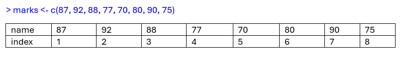
Figure 3.1: Indexing for Numeric Vector

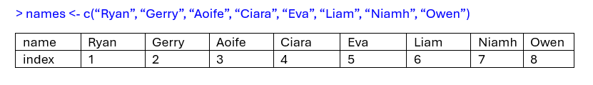
Figure 3.2: Indexing for Character Vector

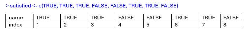
Figure 3.3: Indexing for Logical Vector

This property in vectors means we are capable of extracting specific items from a vector based on their position. If I wanted to extract the first item in my list, I can do this by using [] brackets:

rintro_names[1]

## [1] "Gerry"

Similarly, I could extract the 3rd element.

rintro_marks[3]

## [1] 80

Or I could extract the last element.

rintro_satisfied[8]

## [1] FALSE

This process is called subsetting. I am taking an original vector and taking a sub-portion of its original elements.

I can ask R even to subset several elements from my vector based on their position. Let’s say I want to subset the 2nd, 4th, and 6th elements. I just need to use c() to tell R that I am subsetting several elements:

rintro_names[c(2, 4, 8)]

## [1] "Aoife" "Eva"   "Owen"

rintro_marks[c(2, 4, 8)]

## [1] 65 77 71

rintro_satisfied[c(2, 4, 8)]

## [1]  TRUE FALSE FALSE

If the elements you are positioned right next to each other on a vector, you can use : as a shortcut:

rintro_names[c(1:4)] #this will extract the elements in index 1, 2, 3, 4

## [1] "Gerry" "Aoife" "Liam"  "Eva"

It’s important to know, however, that when you perform an operation on a vector or you subset it, it does not actually change the original vector. None of these following code will actually change the variable rintro_marks.

sort(rintro_marks, decreasing = TRUE)

[1] 91 90 89 88 87 87

print(rintro_marks)
[1] 69 65 80 77 86 88 92 71

rintro_marks[c(1, 2, 3)]

[1] 87 91 87

print(rintro_marks)
[1] 69 65 80 77 86 88 92 71

You can see that neither the sort() function nor subsetting changed the original vector. They just outputted a result to the R console. If I wanted to actually save their results, then I would need to assign them to a variable.

Here’s how I would extract and save the top three exam marks:

marks_sorted <- sort(rintro_marks, decreasing = TRUE)

marks_top <- marks_sorted[c(1:3)]

print(marks_top)

## [1] 92 88 86

3.7.1.3 Vectors - making it a little less abstract.

You might find the discussion of vectors, elements, and operations very abstract - I did when I was learning R. While the list analogy is helpful, it only works for so long before it becomes problematic, mainly because there’s another data structure called lists. This confused me.

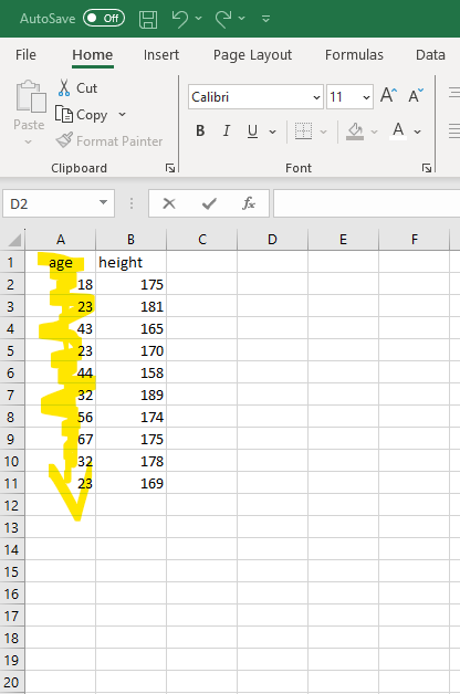
What helped me understand vectors was realising that a vector is simply a “line of data.” Imagine we’re running a study and collecting data on participants’ age. When we open the Excel file, there will be a column called “age” with all the ages of our participants. That column is like a vector in R, containing a single line of data, where every value must be of the same type. For example, a column of ages in Excel becomes this vector in R:

age <- c(18, 23, 43, 23, 44,32, 56, 67, 32, 23)

Similarly, rows are lines of data going horizontally. Imagine, I collect data from another participant (p11). I could represent the data from that individual participant like this in R:

p11 <- c(30, 175)

So whenever you think of a vector, just remember that it refers to a line of data, like a column or a row.

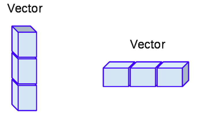
Figure 3.4: Vectors can visually conceptualised as a column or row of data.

What happens when we combine different vectors (columns and rows) together? We create a data frame.

3.7.2 Data frames

A data frame is a rectangular data structure that is composed of rows and columns. A data frame in R is like a spreadsheet in Excel or a table in a word document:

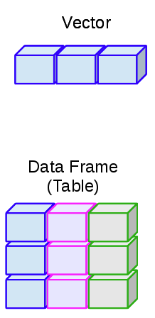
The relationship between data frames and vectors. The different colours in the data frame indicate they are composed of independent vectors

Figure 3.5: The relationship between data frames and vectors. The different colours in the data frame indicate they are composed of independent vectors

Data frames are an excellent way to store and manage data in R because they can store different types of data (e.g., character, numeric, integer) all within the same structure.

Let’s create such a data frame using the data.frame() function:

my_df <- data.frame(
  name = c("Alice", "Bob", "Charlie"), #a character vector
  age = c(25L, 30L, 22L), #an integer vector
  score = c(95.65, 88.12, 75.33) #a numeric vector
)

my_df

##      name age score
## 1   Alice  25 95.65
## 2     Bob  30 88.12
## 3 Charlie  22 75.33

Take a moment and think about what is going on inside data.frame. We have three variables name, age, score. Each of these variables correspond to a different type of vector (character, integer, and numeric). Or in other words, each of these variables correspond to different lines of data. We use the data.frame function to combine these vectors together into a table.

3.7.2.1 Selecting Data from a Data Frame

Once you have created or imported a data frame, you will often need to access it and perform various tasks and analyses. Let’s explore how to access data within a data frame effectively.

3.7.2.1.1 Selecting Columns

Columns in a data frame represent different variables or attributes of your data. Often in data analysis, we want to select a specific column and then perform analyses on it. So how can we individually select columns? Well, in a data frame, every column has a name, similar to how each column in an Excel spreadsheet has a header. These column names enable you to access and manipulate specific columns or variables within your data frame.

We select columns based on their names via two methods:

The $ Notation: You can use a dollar sign ($) followed by the column name to select an individual column in a data frame. For example, let’s select the name column in the my_df data frame:

my_df$name

## [1] "Alice"   "Bob"     "Charlie"

Square Brackets []: This is a similar approach to accessing elements from a vector. Inside the brackets, you can specify both the row and columns that you want to extract. The syntax for selecting rows and columns is: the dataframe[the rows we want, the columns we want].

So if we wanted to access the “age” column of my_df, we could run the following code:

my_df[, "age"]

## [1] 25 30 22

You will notice that we left the “rows” part empty in the square brackets. Leaving this empty tells R “keep all the rows for this column.”

We can also use this approach to access multiple columns using the c() function:

my_df[, c("age", "score")]

##   age score
## 1  25 95.65
## 2  30 88.12
## 3  22 75.33

3.7.2.1.2 Selecting Rows

Rows in a data frame represent individual observations or records. You can access rows using indexing, specifying the row number you want to retrieve, following the syntax: the dataframe[the rows we want, the columns we want].

To get the first row of your data frame (my_df), you can type the following:

my_df[1, ]

##    name age score
## 1 Alice  25 95.65

This time I left the columns part blank; this tells R “please keep all the columns for each row.”

To access the third row:

my_df[3, ]

##      name age score
## 3 Charlie  22 75.33

If you want multiple rows, you can use the c() function to select multiple rows. Let’s select the 1st and 3rd rows:

my_df[c(1, 3), ]

##      name age score
## 1   Alice  25 95.65
## 3 Charlie  22 75.33

If you wanted to select a range of rows, you can use the : operator:

my_df[2:4, ]

##       name age score
## 2      Bob  30 88.12
## 3  Charlie  22 75.33
## NA    <NA>  NA    NA

These methods allow you to extract specific rows or subsets of rows from your data frame.

3.7.2.1.3 Selecting Rows and Columns

We can also select both rows and columns using [] and our syntax: the dataframe[the rows we want, the columns we want].

For example, we could select the first and third rows for the Age and Score columns:

my_df[c(1,3), c("age", "score")]

##   age score
## 1  25 95.65
## 3  22 75.33

Similar to when we indexed vectors, this won’t change the underlying data frame. To do that, we would need to assign the selection to a variable:

my_df2 <- my_df[c(1,3), c("age", "score")]

my_df2

##   age score
## 1  25 95.65
## 3  22 75.33

3.7.2.2 Adding Data to your Data Frame

3.7.2.2.1 Adding Columns

You may often need to add new information to your data frame. For example, we might be interested in investigating the effect of Gender on the Score variable. The syntax for creating a new data frame is very straightforward:

existing_df$NewColumn <- c(Value1, Value2, Value3)

Using this syntax, let’s add a Gender column to our my_df dataframe:.

my_df$gender <- c("Female", "Non-binary", "Male")

#let's see if we have successfully added a new column in

my_df

##      name age score     gender
## 1   Alice  25 95.65     Female
## 2     Bob  30 88.12 Non-binary
## 3 Charlie  22 75.33       Male

Let’s say I noticed I mixed up the genders, and that Bob is Male and Charlie is Non-Binary. Just like we can rewrite a variable, we can also rewrite a column using this approach:

my_df$gender <- c("Female", "Male", "Non-binary")

#let's see if we have successfully rewritten the Gender Column

my_df

##      name age score     gender
## 1   Alice  25 95.65     Female
## 2     Bob  30 88.12       Male
## 3 Charlie  22 75.33 Non-binary

3.7.2.2.2 Adding Rows

What about if we recruited more participants and wanted to add them to our data frame (it is pretty small at the moment)? This is slightly more complicated, especially when we are dealing with data frames where each column (vector) is of a different data type.

What we need to do is actually create a new data frame that has the same columns as our original data frame. And this new data frame will contain the new row(s) we want to add.

new_row <- data.frame(name = "John", age = 30, score = 77.34, gender = "Male")

Once we have this new data frame we can use the rbind() function to add the new row to your original data frame. rbind takes in two data frames and combines them together. The syntax is as follows:

my_df <- rbind(my_df, new_row)

my_df

##      name age score     gender
## 1   Alice  25 95.65     Female
## 2     Bob  30 88.12       Male
## 3 Charlie  22 75.33 Non-binary
## 4    John  30 77.34       Male

There is one important thing to note when adding rows. There must be the same amount of columns as in the original data frame. Otherwise you will get an error. See what happens when I try to add the following new row to our data frame without adding the score column.

new_row2 <- data.frame(name = "Eric", age = 34, gender = "Non-binary")

my_df <- rbind(my_df, new_row2)

## Error in rbind(deparse.level, ...): numbers of columns of arguments do not match

my_df

##      name age score     gender
## 1   Alice  25 95.65     Female
## 2     Bob  30 88.12       Male
## 3 Charlie  22 75.33 Non-binary
## 4    John  30 77.34       Male

The names in this error message refers to the names of the columns (in this example, name, age, scores, and gender). Since our new_row2 is missing a column name that is in my_df, we cannot add this row to the column.

But what if we don’t have a score for Eric? Is there no way to add his result to our data frame? There is. All we need to do is add the column score in our new_row2, but give it the value of NA. The term NA basically means Not Available - as in we don’t know the value for this variable.

new_row2 <- data.frame(name = "Eric", age = 34, score = NA, gender = "Non-binary")

my_df <- rbind(my_df, new_row2)

my_df

##      name age score     gender
## 1   Alice  25 95.65     Female
## 2     Bob  30 88.12       Male
## 3 Charlie  22 75.33 Non-binary
## 4    John  30 77.34       Male
## 5    Eric  34    NA Non-binary

NA values can be quite common in real life datasets - sometimes data goes missing! But we’ll come back to the concept of NA later on in this course and we will learn a variety of ways to deal with them.

3.8 Summary

That concludes this session. Well done, we did a lot of work today. We learned more about the relationship between the console and the script and how we need to be precise when writing commands. We introduced the different types of data that R stores and how those data types can be stored in single lines of data in vectors or combined together in a table in a data frame.

Don’t feel like you need to have mastered or even remembered all the material that we covered today. Even though these concepts are labeled as “basic,” that does not mean they are intuitive. It will take time for them to sink in, and that’s normal. We’ll drill these concepts a bit further next week. We’ll also learn how to import data frames, which will set us up nicely for working with the type of data sets we see in Psychological research.

3.9 Glossary

This glossary defines key terms introduced in Chapter 3.

Term	Definition
Assignment	The process of assigning a value to a variable using the assignment operator (`<-` or `=`).
Character	A data type representing text or strings of characters.
Data Frame	A two-dimensional data structure in R that resembles a table with rows and columns. It can store mixed data types.
Data Type	The classification of data values into categories, such as numeric, logical, integer, or character.
Element	An individual item or value within a data structure, such as a character in a vector.
Index	A numerical position or identifier used to access elements within a vector or other data structures.
Indexing	The process of selecting specific elements from a data structure using their index values.
Integer	A data type representing whole numbers without decimals.
Logical	A data type representing binary values (TRUE or FALSE), often used for conditions and logical operations.
Numeric	A data type representing numeric values, including real numbers and decimals.
Object	A fundamental data structure in R that can store data or values. Objects can include vectors, data frames, and more.
Subsetting	The technique of selecting a subset of elements from a data structure, such as a vector or data frame, based on specific criteria.
Variable	A named storage location in R that holds data or values. It can represent different types of information.
Vector	A one-dimensional data structure in R that can hold multiple elements of the same data type.

3.10 Variable Name Table

Rule	Type	Incorrect Example	Correct Example
Variable names can only contain uppercase alphabetic characters A-Z, lowercase a-z, numeric characters 0-9, periods ., and underscores _.	Strict	1st_name	first_name
Variable names must begin with a letter or a period.	Strict	_1stname	.firstname
Avoid using spaces in variable names.	Strict	my name	my_name
Variable names are case-sensitive.	Strict	my_name == my_Name	my_Name == my_Name
Variable names cannot include special words reserved by R.	Strict	print	to_print
Choose informative variable names that clearly describe the information they represent.	Recommended	money	income
Opt for short variable names when possible.	Recommended	date_of_birth	dob
Prioritize clarity over brevity.	Recommended	tem	total_exam_marks
Avoid starting variable names with a capital letter.	Recommended	FirstName	firstName
Choose a consistent naming style and stick to it.	Recommended	myName, last_Name	my_name, last_name or myName and lastName

Including the “>” is a pain when formatting this book, so I won’t include “>” in examples of code from this point forward.↩︎
If you do not know what a p-value is, do not worry. We will introduce this concept later and discuss it extensively.↩︎
I used the function rnorm() to generate these values. If you want to read more about this very handy function, type ?rnorm into the console, or follow this link.↩︎